
Taking over the world
But first you need a map

One of my favorite shows was Pinky and The Brain when I was growing up. In each episode, Brain hatches a plan to achieve his goal of world domination, a plan that inevitably fails, often due to his arrogance. Our robot has different (peaceful!) goals, and as far as I can tell, it isn’t arrogant. It will however have a hard time succeeding if it can’t navigate its surroundings. Before we cover navigation, let’s zoom out a little. Here are the capabilities our robot needs, along with the supporting software and hardware components:
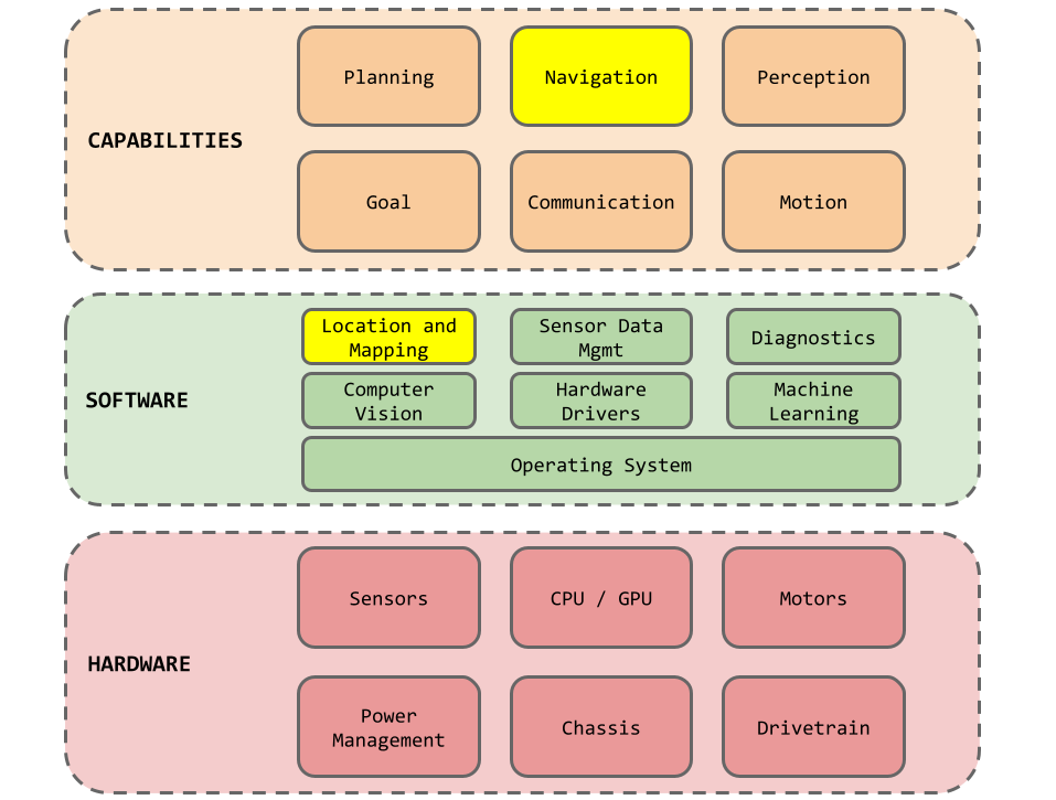
This diagram summarizes the core capabilities that our robot needs to accomplish its task. It also illustrates that capabilities are built on top of software that works with the hardware to sense and act.
Navigation
Now lets talk about Navigation, highlighted in the yellow parts of the diagram above. Navigation means building a map of our robot’s environment, and determining the robots position on the map. Our robot needs to navigate a changing environment (e.g. lighting conditions or encountering a new obstacle). Our robot should also be able to map all reachable areas and shouldn’t miss any spots. Fortunately, there is an approach that ticks all the boxes: SLAM.
What is SLAM?
SLAM (Simultaneous Location and Mapping) is a technique that uses sensors like LiDAR (lasers that fire light pulses) or video cameras to build a map and determine the robots position in real time. ‘Real time’ means the map is updated quickly enough for the robot to recognize changes in the environment (e.g. opening a door) and adapt accordingly.
How does it work? The general approach is summarized below:
Record what the sensor ‘sees’. This involves processing the raw data generated by the sensor and For example, LiDAR generates coordinates for objects in the environment by emitting lots of laser pulses and measuring how long it takes for each pulse to return to the robot. An (x,y,z) coordinate representing the location of the environment object is generated. There are thousands of these coordinates which constitute a point cloud.
Update the position when the robot moves. As the robot moves, the sensor measures the environment. The new sensor data is compared to previous sensor data (the existing map) to determine the robot’s position and orientation.
Errors in the robot’s location can accumulate and need to be managed. This can be done by keeping track of previously visited landmarks and using them to recalibrate.
There are many different variants of SLAM that use different algorithms (filters/graphs/deep learning), sensors (LiDAR, sonar, video, inertial), and how much visual intelligence is used to understand the scene.
The most likely candidate for our robot is vSLAM, a version of SLAM that uses video cameras. Distance estimation is not as accurate as LiDAR, but it’s much less expensive, and offers much more visual data to build a semantic understanding of the environment.
This hopefully gives you a taste of SLAM. It’s a very deep topic, and one we’ll be revisiting as our robot progresses.
Progress
It’s been a short week as we were traveling last Friday. Most of this week has been spent focusing on the Deep Learning for Computer Vision course CS231n. The first 4 lectures covered the following:
linear and kNN classifiers - to predict which class an image belongs to
loss functions - to quantify the quality of the model weights
regularization - to prevent a model from overfitting to the training data so it makes better predictions for new data that isn’t necessarily like the training data)
optimization - to determine model weights that minimize the loss function using gradient descent
neural networks and backpropogation - on to the exciting stuff! Multi layer neural networks are non-linear classifiers that enable more complex boundaries to more accurately separate off classes of data points from other classes.
Analytically calculating the optimal weights (that minimize the loss function) for these networks is hard and resource intensive (huge matrices) so lets not do that. Instead:
Represent the network as a computational graph, where each node is a neuron
Use the chain rule to calculate how changes in each neuron’s inputs (upstream gradients) affect it’s outputs (downstream gradients).
back propagation: Apply the chain rule recursively along the graph to compute gradients of all inputs/parameters/intermediates. Compute the gradient of the loss function wrt the inputs.
It’s not all slides and lectures. I’ve been implementing linear and kNN classifiers in NumPy and enjoyed implementing a fully vectorized version of a loss function that resulted in a 100x speed up on my M4 mac mini!
Links
These papers highlight differences between artificial neural nets and biology: