
Making Computer Vision Stick
Reconstructing the first 3 lectures of CS231n

Richard Feynman says memorizing a bunch of facts, or dissecting the terms of an equation doesn’t mean you understand something. The real test is whether you can explain it in your own words and minimize the jargon. In that spirit, I’ll share what I’ve learned in the first 3 lectures of CS231n.
Warning! This is a long post and there’s math involved. If that’s not your jam, then skip to the end to check out some cool links.
Computer Vision - what’s it good for?
The goal for computer vision is to enable a machine to make sense of visual information. ‘Make sense’ means:
classifying different elements of an image or video
knowing their names
relationships between the elements, like a person walking their dog
understanding intent and context so we know if an image is funny, if someone is doing something dangerous, navigating through an obstacle course
Computer vision does #1 and #2 well, struggles with #3, and has a ways to go for #4.
The class has focused on item #1 for the first 3 lectures. That makes sense - you need to classify images properly before you can do anything else.
Classification - overview
How does classification work? Generally speaking:
Start with a set of correctly classified images, called the ‘training set’
Use the training set to train a model
Run an image through the model which assigns a class to it. We call this a prediction because we don’t know if the model is right.
Determine how wrong the prediction is by using a ‘loss function’
Use the output of the loss function to adjust the model so it is less wrong next time.
Naive ways to classify an image
The first two approaches we covered are Nearest Neighbor (NN) and an extension of it, called k Nearest Neighbor (kNN). These use only the first 3 steps outlined in the previous section. Also, training step (step 2) is super easy because there’s not much training to speak of: the model is ‘trained’ by having copy of every test image. So let’s talk about how they work.
Naive approach 1: Nearest Neighbor
This classification approach is pretty simple. Each of the test image’s pixels is compared to the corresponding pixel in a training image by calculating the average manhattan (L1) or euclidean (L2) distance between the pixels. Repeat for all images in the training set. The test image is classified to the closest training image - the one with the lowest distance score.
Problems with this approach include:
Two wildly different images can be incorrectly assigned to the same class if they are mostly the same color (e.g. lighthouse near the sea and a boat in the say).
Does not handle cases where the same images has different lighting/orientation/zoom conditions.
It’s super fast to train but storing all training images takes a lot of memory. Even worse, predictions take a lot of time because the each test image is compared to all images in the training set. Yuck.
Accuracy on the CIFAR data set is 27% so nothing to write home about.
Naive Approach #2: k Nearest Neighbor
This approach builds on the previous one by using the n closest scores and tallying their classes as a sort of popularity contest; pick the class with the most votes and assign it to the image you’re trying to classify.
Accuracy is incrementally better than NN, with ~28% accuracy on CIFAR for k = 5.
Jargon alert: hyperparameters, cross validation and more
The first time I encountered hyperparameters, I pictured a bunch of parameters that ran around yelling and waving their arms. The reality is much more boring (peaceful?). Parameters are the things that are set during training. Hyperparameters on the other hand, are set before training starts. The ‘k’ in kNN is an example of a hyperparameter, as is the choice of function to calculate distance between images (L1, L2, etc).
How do you pick a value for a hyperparameter like k? You test out a few different values and pick the one that gives the best results. There’s a problem though. Your test set is like a beautiful engagement ring - rare and precious. You want to save it for your one true love, and in our case that means saving the test set for the final validation phase, after the optimal k value has been chosen. Otherwise, you’ll choose a hyperparameter that works well for the test set, but bombs out on new images.
How do we handle this? Well, we can’t touch the test set, so that leaves the training set. We split the training set into two parts (called folds) consisting of a slightly smaller training set, and a small validation set that we treat as a fake test set (remember what a test set is for?) to tune the hyperparameters. Using our trusty CIFAR training set as an example, we might shrink the training set from 50,000 images down to 49,000 and use the remaining 1000 images for validation.
There’s another problem if your training set (and associated validation set) are small because it becomes super important to choose a representative validation set. Fortunately there’s a way to use all of the training set as a validation set. You do this in a piecemeal fashion: first by evaluating against the validation set, then eval against a new validation set picked from a different part of the training set, and repeat until all of the training set has been pressed into service as a validation set. Lastly, average the interim eval scores to get the final score. This process is called cross-validation.
Here’s an example: split the training set into 5 equal folds. Use the 1st fold for validation, and the remaining 4 as the training folds. Eval the training folds against the validation fold to get an interim eval score. Repeat with the 2nd fold as validation and the other 4 folds as training, until you’ve used every fold for validation. Take the average at the end. Here’s an illustration:
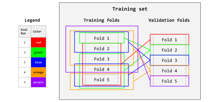
These steps are repeated for each value of hyperparameter you want to test. As a result, cross-validation is computationally expensive. Use it only when necessary - typically when each fold is a few hundred images.
Let’s move on to fancier classifiers.
Linear Classifiers
Okay, now we move to a classifier that uses all 5 elements from our overview. This approach extends beyond Linear Classifiers to neural networks so its worth breaking it down to make sure we understand it really well.
What is a linear classifier? It’s a classifier that applies a linear function to an image to predict its output class.
W and b are parameters that are applied to a training image xᵢ to give a prediction. What does that mean really? Let’s start with terms. I’ve added in values [in brackets] from the CIFAR-10 dataset, a collection 50k categorized images, to make things concrete:
1. There are N images in the training set. [N = 50,000]

2. An image can be classified in one of K categories. [K = 10]

3. xᵢ is the i’th image in the training set, consisting of D pixels. It is represented as a [D x 1] column vector. [D = 32x32x3 = 3072]

4. Not referred to above is yᵢ which is the label associated with xᵢ.

5. W is a weight matrix, a matrix of size [K x D].

6. b is a bias vector, a column vector of size [K x 1].

7. f() is the score function.
Here’s a nice example from the CS231n notes, modified to use different colors that are less likely to be mistaken as RGB pixel values. To simplify things, the image is now 4 monochrome pixels (D=4) and there are only 3 categories (K=3).
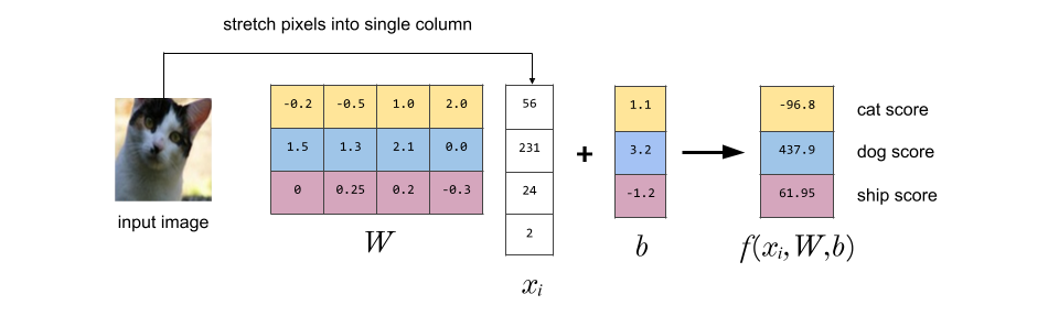
You can think of each row of W as a classifier for one of the classes (e.g. the top yellow row of W is the ‘cat classifier’).
To see why we need the bias vector b, think of each pixel of an image as a dimension (so 4 dimensions in our example). So each image can be represented as a point on a 4 dimensional grid. A linear classifier classifies images by drawing lines/planes/hyperplanes (depending on the # of dimensions) to break up the 4D space into classes. Changing a row of W rotates this line/hyperplane around, but without the bias vector, each line/plane/hyperplane would have to go thru the origin. So the bias vector lets us move our dividers around.
I’m not biased
We know now why a bias vector is useful but it’s kind of annoying to track. Fortunately we can incorporate it into W by smushing b onto the end of W and appending a ‘1’ to our image data:
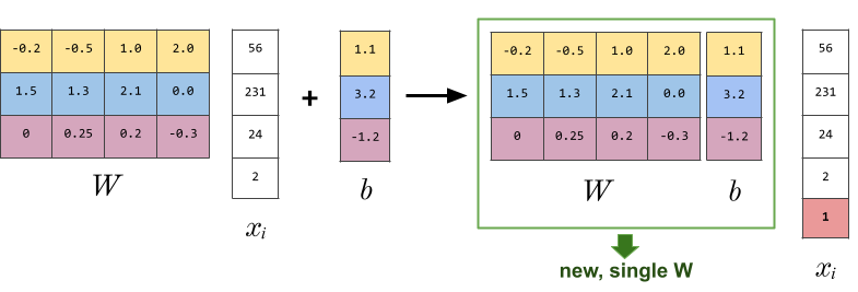
Now we have only a single matrix to worry about. Going back to our CIFAR-10 example, D is now 3072+1 = 3073, and W is now 10 x 3073.
A losing proposition
Look back at figure 1 (I’ll wait). Notice something? Our genius classifier thinks our cat is a dog. Before selling our Nvidia shares in a panic, lets try adjusting the weights (W) to see if that helps. But what to adjust them to? That’s where loss functions come in.
How does a loss function work? Let’s have a student Wally represents our weights (W). Wally is taking an exam to classify images (X). He writes down which class each image belongs to, and he also writes how confident he is about his answer. Louise is Wally’s teacher, and represents our loss function (f). She uses the following marking scheme to grade his exam:
Right answer, high confidence that answer is correct: 4 marks
Right answer, low confidence that answer is correct: 3 marks
Wrong answer, low confidence that answer is correct: 2 marks
Wrong answer, high confidence that answer is correct: 1 mark
Well, almost. I’ve left something out - the marking scheme is actually reversed. So a right answer/high confidence gets a 1, and the wrong answer/high confidence gets a 4. You see, Louise has developed a bitter streak after years of teaching, and prefers grading how unhappy she is with each answer. Poor Wally gets his exam back and is excited to see a high score on his exam…until he realizes lower scores are better.
Like Louise, a loss function measures our unhappiness with predictions on the training set. Low scores are better!
What does a loss function look like? Let’s take a look at a couple of them.
Multiclass Support Vector Machine (SVM) Loss
SVM is our first loss function. It wants a classifier that picks the right class for every image and be confident in its choice. What does that mean?
Start with the i’th training image xᵢ along with its correct class in yᵢ. Then the score function f(xᵢ, W) takes xᵢ’s pixels to calculate the class score for every class. The scores are in a vector s, where sⱼ means the j’th element of s (score for the j’th class). Assigning a large score to a class means the classifier is confident its found the correct class for the image. Assigning a smaller score to a class means the classifier is confident the class isn’t the right one.
So how does our SVN grade our scoring function? It wants the score for the right class for an image to be bigger than the score for a wrong class. How much bigger depends on a hyperparameter called 𝝙. This can be safely set to 1, and we’ll see why when I cover the concept of regularization in the next section.
If the SVN gets what it wants, there is no loss, and so the loss value stays the same. Otherwise, the margin and the difference between scores is added to the total loss (remember, a lower loss is better). Here’s the equation for our SVM loss function:
The term inside the sum is known as a hinge loss.
Too many solutions
Recall our linear classifier:
Also recall that we tweak the weights in W to improve its accuracy (I know I haven’t explained how yet…we’re getting there!). And lets say we do such a great job setting W that SVN gives a loss of zero. Perfect! Until we realize there might be other Ws that give the same result.
Continuing with the perfect SVN, scaling W by a number gives us the same zero loss. To see how, remember that the zero loss for an image is because each wrong class score is bigger than the right class score by 𝝙. Multiplying W by 2 for example will scale all of the class scores by 2. Double the wrong class score minus double the right class score exceeds the margin 𝝙 by even more than before, giving a zero loss.
So our example has lots of Ws that work. What’s the problem? The problem is that the influence of the largest weights in W increases as you multiply W by larger numbers. Since the class score is calculated by multiplying the weights by the image pixels (dimensions), you risk giving a few dimensions an outsize influence on the score.
But you might say - okay, who cares? We still get a zero loss, right? That’s true, but remember, we are working with training images. When you feed in new images, the scaled up weights don’t generalize well and perform poorly with new data. W overfits the training data. Now that we have a handle on the problem, lets look at a solution.
Regularization
Regularization doesn’t make an ideal song lyric1 - it just doesn’t roll of the tongue very easily. But that’s cool, because it solves the overfitting problem by reducing the influence of large weights in W. No tall poppies here!
We cut W’s tall poppies down to size by applying a regularization penalty to each of its weights. The penalty is usually calculated by using the squared L2 norm, and its size is controlled by yet another hyperparameter (ƛ) called the regularization strength. Here’s what that looks like.
We add this term to our loss function L which now has two terms: data loss (the original term) and the new term, called regularization loss. The loss function looks like this:
This calculates the loss for one image. For the full loss we have to consider the losses for all images in the training set. We do that by calculating the average data loss for all images, resulting in the complete multiclass SVM loss:
One more thing. Earlier, I had said it was okay to set Δ to 1.0. That’s because the hyperparameters ƛ and Δ control the same tradeoff: how much influence each term has on the loss score. To see why, notice that shrinking Δ shrinks the data loss score. Similarly, shrinking ƛ reduces the regularization loss score. So you can reduce either of these to reduce the complete loss L. Recognizing this, we set Δ to 1.0 and adjust the regularization strength ƛ to control how much we allow the weights in W to grow.
Softmax Loss
SVM is fine, but it spits out loss scores that are hard to interpret. Enter the softmax function, which converts the scores into probabilities:
This looks intimidating but all it does is take a bunch of loss scores like 239.2 or -12.9 and squishes them to between 0 and 1 so that if you add them all up, you get 1.
Here’s what it looks like in our loss function where fⱼ is the j-th element in vector f of our class scores:
Notice in the first equation that the softmax function is wrapped inside a -log() function. Remember that SVM used a threshold to calculate the loss, which was called the hinge loss. You can’t do that, because softmax turned the scores into a bunch of probabilities between 0 and 1, right? So we have to these scores differently, by using a cross-entropy loss, and that’s where the -log() comes from. This post is already super long, and there’s one more topic to cover, so I’ll explain cross-entropy loss next time.
Practical matter: Calculating the exponentials in our loss function can cause an overflow. To work around this, subtract the max value in f from each element, shifting their values down so the largest number is 0.
Before we move to our final topic for today, let’s check in on our hapless student Wally. After several therapy sessions, he’s come to terms with failing his classification exam. He’s ready to learn from his exam to do better next time. But he’s not sure how. Our classifier is in the same boat as Wally: the loss function indicates how unhappy we should be with our classifier’s results. How can we use what the loss function tells us to improve our classifier?
Optimization
To review, the core of our linear classifier is W, made up of parameters called weights. L is a loss function that gives a loss score for the quality of the weights. We want to tweak the linear classifier to reduce the loss score (remember lower loss scores are better). That means adjusting the weights in W, since that’s the only part we can change.
So we want to find the weights that give the lowest loss score. There are many possible weights, and it would take forever to try them all so we need to try something else.
We could make small random changes to the weights, but that’s not efficient either. Instead, think of each weight in W as a dimension (10x3073 is 10,370 dimensions) in a loss landscape, and you can take a step in any direction in this landscape by making a small incremental change to some or all of the weights. For each step, you want to step in the direction that reduces the loss score compared to your current location. But how?Just follow the gradient.
Follow the yellow brick gradient
For our purposes, a gradient points in the direction of steepest descent in our loss landscape. You calculate this by taking partial derivatives of the loss function along each dimension resulting in a vector of partial derivatives for each dimension. This vector points to the direction of steepest ascent. But you want to go down, not up so turn around 180° by negating the direction vector. Then take a step in that direction by multiplying it by your step size. Then add the result to W (‘parameter update’).
There are two ways to calculate the gradient :
Incrementally. We step forward in one dimension at a time and calculate how much the loss score changes along that dimension. That is easy to calculate, but it’s kind of lame because you have to calculate L for every dimension (10,370 times) for each parameter update.
Analytically. It’s much faster if you have the equation for the gradient, since you can calculate the gradient for all the dimensions at once. But it’s a pain to derive, especially if it’s been a minute since you’ve taken calculus.
The overall process is called gradient descent and it looks like this:
Calculate the gradient L for W (analytically or iteratively).
Update the paramter W to step in the direction L is dropping fastest.
Repeat until improvements to loss score are minimal/gradients aren’t changing/weights aren’t changing.
Practical points: It’s easy to make mistakes with the analytic approach, so check it with the iterative approach too. Choosing a step size involves trial and error; too small and progress takes forever; too large, and you may miss the optimal solution.
Phew! That’s it for this week - congratulations if you’ve read (or skimmed) this far!
What I’ve Been Reading/Watching/Listening to
The State of AI, November 2025: Benedict Evans released the latest version of his semi-annual monster slide deck covering the latest macro trends. I’ve enjoyed his thoughtful analyses for more than a decade. This deck is a must read for anyone trying to understand where AI is, and where it might go.
Benedict confirms what I believe - that AI is a technology shift as big as the PC/internet/mobile revolutions I’ve experienced. Is it bigger than fire? People like warmth, so that’s a pretty high bar.
The Thinking Game. An engaging documentary about how Demis Hassabis and his team at Google DeepMind used AI to solve protein folding, a problem that scientists had been trying to solve for 50 years with little success. I wish they had gone into more technical details, but I enjoyed the biographical bits and it gives the layperson an idea of how AI is impacts science.
Elon Musk interviewed by Nikhil Kamath. I wasn’t sure what to expect, but it was a good interview. Lots of personal bits, but the relevant takeaway is that he believes robotics + AI are a big deal and will change society in profound ways (you won’t need to work, unless you want to. money goes away). I obviously agree with the first part , but I’m doubtful about the second part. Any big technology shift makes some jobs obsolete (newspaper delivery), while creating new ones (Youtube influencer).
Tangle. Shopify open sources a platform to streamline and speed up ML experimentation. Teams visually build data or ML pipelines that run locally (Docker/podman) or in the cloud (Huggingface). Workflows are specified declaratively (vs. code) and let you track package dependencies which makes it easier to reproduce experiments.
Deep Reinforcement Learning for Robotics: A Survey of Real-World Successes. This research paper evaluates how effective RL is for locomotion, navigation, object manipulation, and interaction. There’s a lot to like here. The robotic capabilities covered are relevant to our prototype. It’s recently published, so it’s an up to date snapshot. And last but not least, the authors measure an approach’s effectiveness by considering real world deployment which is obviously a relevant yardstick for us. I’ll be referring back to this as design and development progresses.
NeurIPS 2025 - The big annual AI & ML research conference took place this week, and there are a few workshops that look relevant for the prototype. I’m capturing them here for future reference.
Embodied and Safe-Assured Robotic Systems covers topics like ‘robust robotic perception in dynamic/uncertain environments’.
Vision Language Models: Challenges of Real World Deployment covers topics like making VLMs run efficiently on embedded systems, and effective training for tasks in visual scenes.
Sub for free updates.